Forecasting Energy Demand Using Time Series AutoML

Read time: 8 minutes

Hey there,

Saving energy is more important than ever.

Today's use case will focus on time series forecasting as a means of predicting energy demand and optimizing energy production.

Time series forecasting is a powerful method for predicting future events based on prior data. AutoML services can help us in this task, as they can process large amounts of data and quickly identify patterns in it.

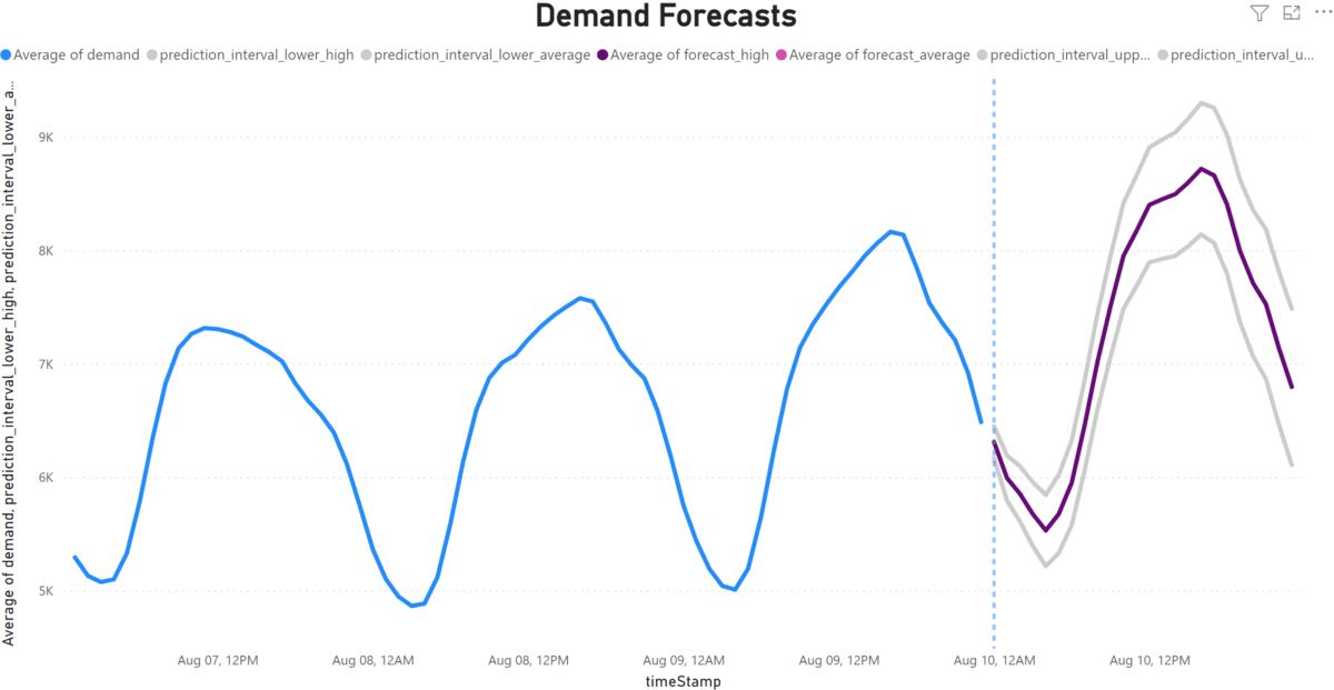
Here's the dashboard we're going to build:

Let's go!

The winners of the book raffle have been announced! Take a look at the comments:

Problem Statement

Let's say we're working for an energy company that wants to forecast the energy demand for New York City over the next 24 hours.

Our existing BI dashboard on historic data suggests that the weather could have an effect on the total energy demand:

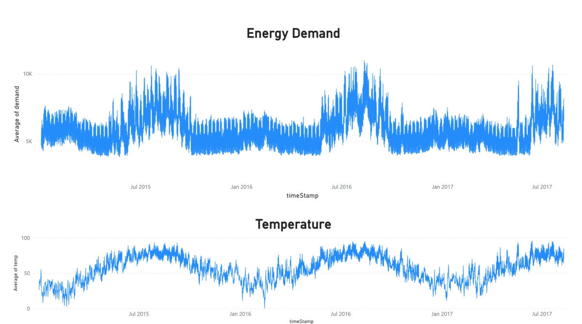
That's why we want to try to incorporate weather data to improve the accuracy of our predictions over the next 24 hours.

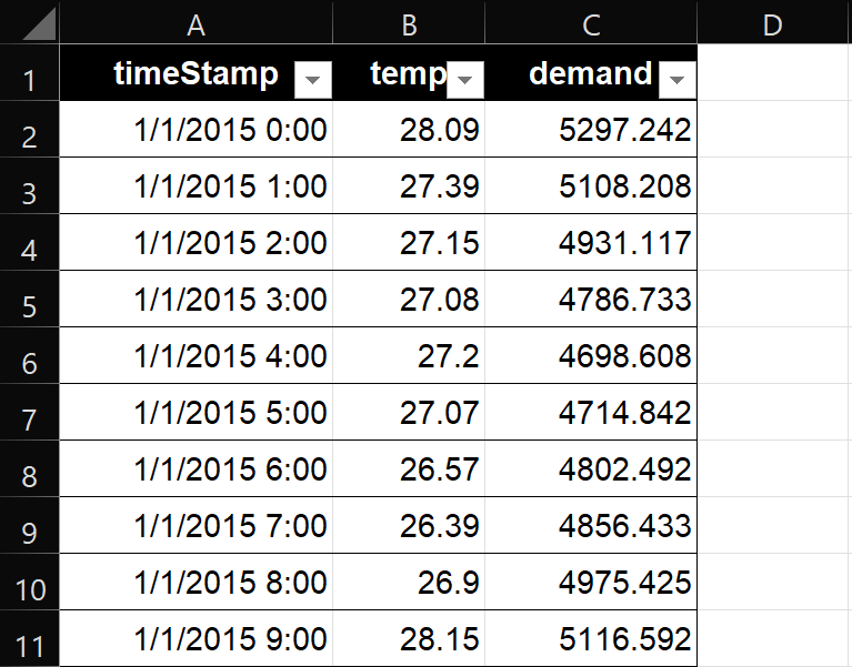
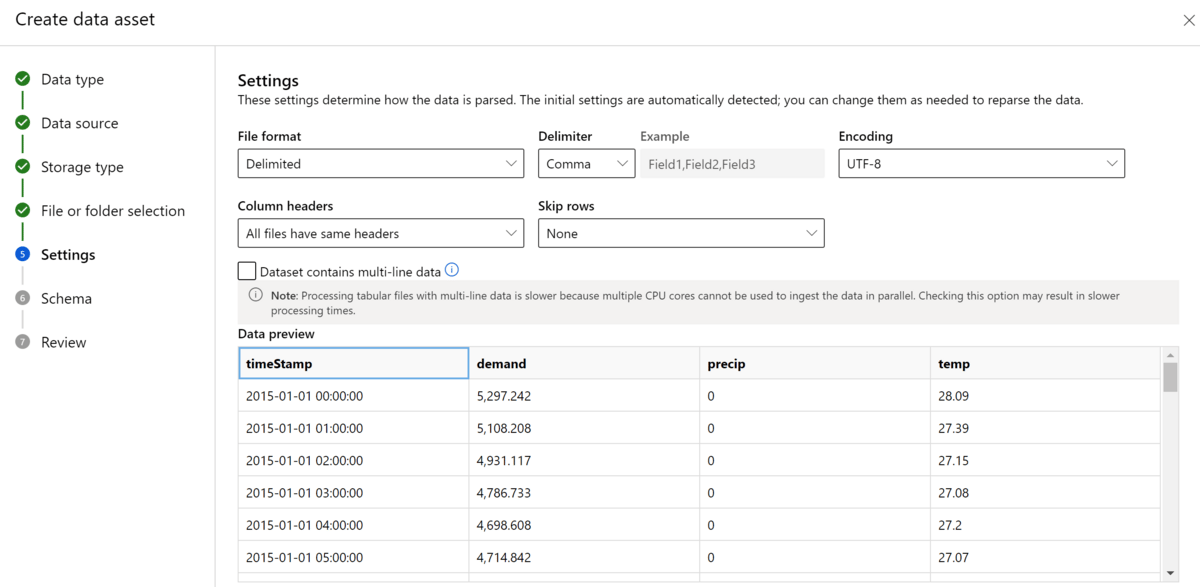
We have access to energy demand data and weather data from the past 2.5 years at an hourly interval - that's more than 22,000 rows of data looking like this:

Here's how we tackle this:

Solution Overview

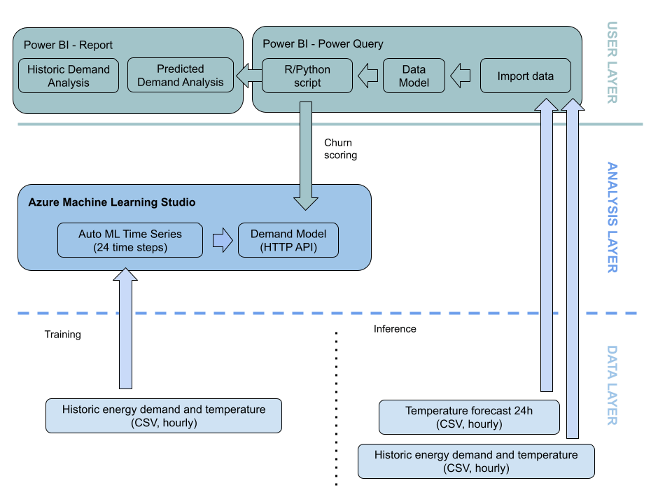
Take a look at the overall use case architecture and the three layers: Data - Analysis - User.

We'll go through these layers step by step:

Data Layer - Training

Our training data consists of hourly measurements of New York City's energy demand and temperature data for the past 2.5 years - more than 22,000 rows of data in total. With this data, we'll train a machine learning model that can predict New York City's energy demand for the next 24 hours given a recent temperature forecast.

Data Layer - Inference

For prediction, we use the most recent temperature forecast for the next 24 hours which will serve as the input to our model. We'll also make the historic data available to our BI software so we can show the historic data as well.

Analysis Layer

To build the model, we use a combination of time series prediction algorithms on Microsoft Azure's AI platform and AutoML capabilities. We chose AutoML to take advantage of automated feature engineering and hyperparameter optimization for better accuracy and performance.

User Layer

We'll show the predicitons in Microsoft Power BI - but any other BI tool would work as well.

Power Query does the data processing for us. We use a small Python or R script within Power Query to send the weather forecast data to the hosted model API, retrieve the demand predictions, and integrate them into our data model.

The final Power BI report will be a line chart that shows the actual energy consumption over the past 48 hours and the forecast for the next 24 hours with the upper and lower confidence bands of our prediction.

Model Training on Azure ML Studio Walkthrough

Navigate to ml.azure.com, select Automated ML and choose "New Automated ML job". Create a new dataset and upload the file "nyc_energy_demand.csv" which is linked in the resources below. The dataset preview should look like this:

Next, create a new experiment named "energy-forecast". Select "demand" to be the target column and select a cheap compute instance.

Select "Time series forecasting" as the machine learning task. Enable autodetect for time series identifiers and frequency. Set forecast horizon to 24 since each time step in our training data is one hour and we want to predict the next 24 hours. Keep deep learning disabled for now.

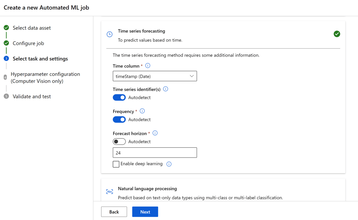
You can leave on cross-validation with autodetect options for step size and number of folds. Click Finish.

While the AutoML process is running (about 30 minutes), check the output of the models that have been generated.

You can explore each model and inspect its performance (select model → Metrics).

For example, here's a model that only predicts the average of the time series (who said AutoML is always fancy?)

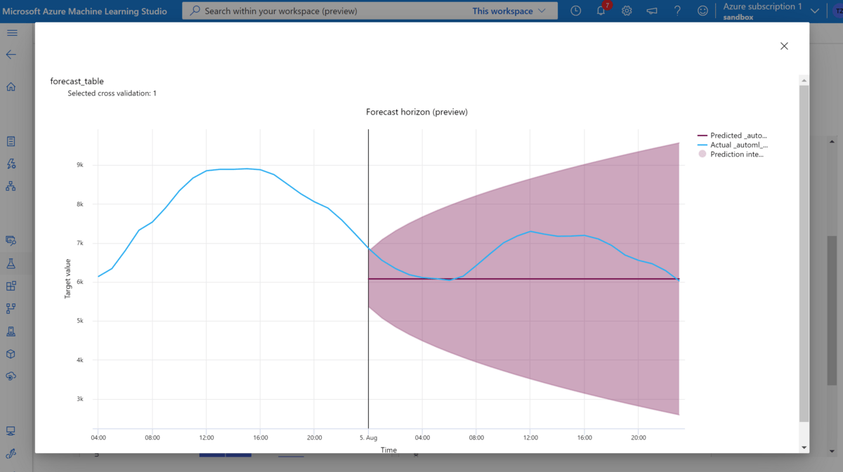
Of course, that's not really helpful.

AutoML produces more advanced models as well such as this one over here which predicts the seasonal average:

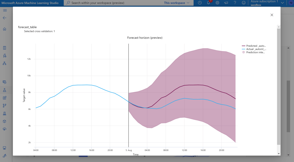
We're getting closer!

The best model (lowest normalized root mean squared error) finally turns out ot be a VotingEnsemble with a Normalized RMSE of 0.038.

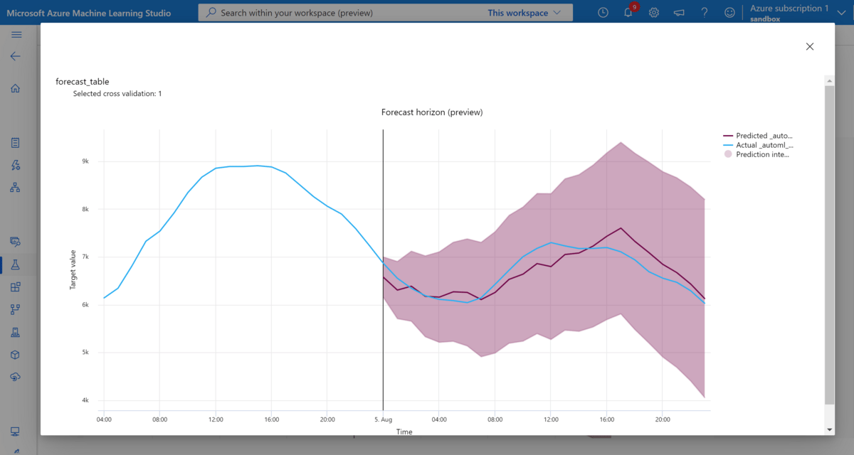
We can see how the predictions are pretty good at the beginning of the new time series and get worse as we look further into the future. This is typical for time series forecasts.

Whether or not this prediction quality is good enough depends on our use case and the existing baseline we've got. If all we had was a simple moving average before, than this model would be far better.

Let's deploy this model (Model → Deploy → Web service).

Once the deployment is complete you can see your model in the endpoints and test from the web GUI (Endpoints → Select Endpoint → Test). For example, let's enter some weather forecast data and see what the model predicts:

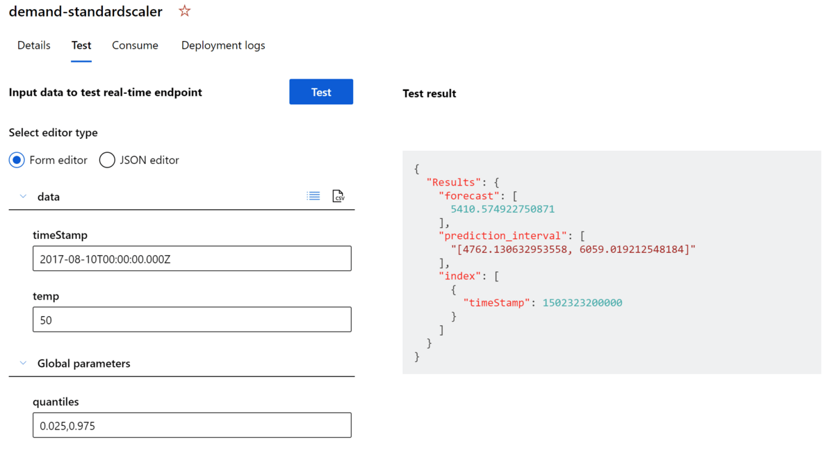
Seems to work as expected! Given a date (which is newer than the training data) and a temperature value we get a forecast for the energy demand as well as the interval for our confidence bands.

Now how can we integrate this into Power BI or any other BI tool?

All we need to do is query the online API under which the model is hosted (there are other methods, such as writing the results to a database).

For now, let's continue with the online prediction and call this API from Power BI.

Power BI Walkthrough

To follow allong, open Demand-Forecast.pbix file in Power BI dashboard.

Power Query

In Power BI Desktop, navigate to your data model and open Power Query. Power Query lets us manipulate the data and will also serve as the glue for our workflow.

In Power Query, we add the following steps to our weather forecast table:

• Fix data types (convert dates back to string for better handover to R/Python)

• Run R or Python script (sends weather data to API and fetches results)

• Turn date column back into datetime format

• Rename colums for better readability

You can see that our table now contains the new columns with the forecasted demand and prediction intervals:

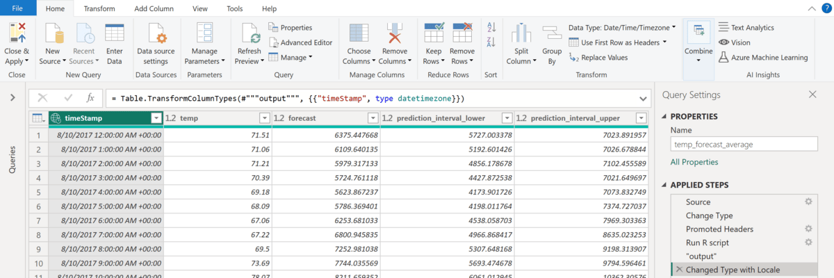
Hit Save & Apply and continue to the report editor to build our dashboard.

Report

Create a new report page called Forecast.

Pull a line chart on the canvas which has timeStamp on the x-axis and Average of demand, prediction_interval_lower, prediction_interval_higher and average of forecast on the y-axis.

With a little styling, we can make this chart look similar to this:

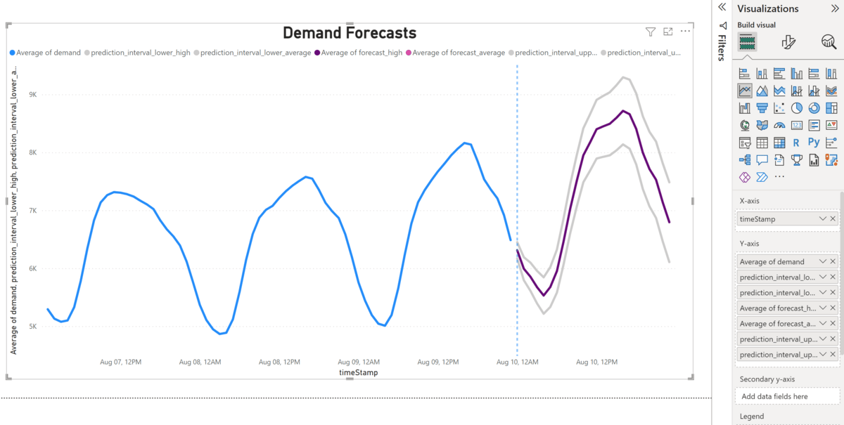
The blue line shows the historic data.

The purple line shows our predictions and the grey lines show our confidence bounds.

We could even take this a little furter and show forecasts for different scenarios: 

Suppose instead of only one we get two weather tables - one with a conservative forecast and the other with a riskier forecast.

We could now get inference from our model for both weather tables and include them as two separate measures, allowing us to switch between two scenarios with a filter or display both scenarios in one graph:

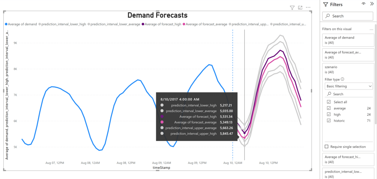
So this dashboard gives us a good overview of the expected energy demand in the next 24 hours - both for a conservative scenario and for a more risky one.

Conclusion

Today's use case showed how we can use AutoML to create a quick prototype for demand forecasting.

While this implementation is far from production-ready, it gives us a good first indication of how good an AutoML time series forecast would perform on our data.

If we already had a time series forecast, we could simply run this dashboard in parallel and see how it performs.

As we get new data, we can re-train our model - a process that can be easily automated on Azure.

I hope this use case has sparked your creativity and given you some more ideas!

Feel free to recreate this exercise using the resources below.

See you again next Friday!

Resources

• Download the dataset, scripts and Power BI file

If you liked this content then check out my book AI-Powered Business Intelligence (O’Reilly). You can read it in full detail here: https://www.aipoweredbi.com