Understanding Evaluation Metrics for Predictive Analytics

Hey there,

Today, I want to give you an overview of the key concepts and metrics you need to properly evaluate your predictive models.

Evaluating model performance is critical to determining whether your models are accurate, working as intended, and providing useful predictions.

We'll cover the key metrics for evaluating both regression and classification models so you can confidently evaluate your models and make data-driven decisions.

Ready? Let's go!

You can't predict what you can't evaluate

Predictive analytics is all about finding a model which has a good trade-off between prediction errors on data from the past and prediction errors in the wild on new data.

No matter how you build these models - using AI, machine learning, or even by hand - understanding evaluation metrics is critical as they help us to:

• compare models to one another to find the best predictive model

• continuously measure the model’s true performance in the real world

The basic idea here is very simple: we compare the values that our model predicts to the values that the model should have predicted according to a ground truth.

What sounds intuitively simple carries a good amount of complexity.

The first thing to know is that the evaluation metric you choose depends on the predictive problem you're trying to solve - whether it's a regression or classification problem.

Evaluating Regression Models

Regression models predict continuous numeric variables such as revenues, quantities, and sizes. The most popular metric to evaluate regression models is the root-mean-square error (RMSE).

RMSE

It is the square root of the average squared error in the regression’s predicted values (ŷ).

The RMSE can be defined as follows:

RMSE measures the model’s overall accuracy and can be used to compare regression models to one another. The smaller the value, the better the model seems to perform.

The RMSE comes in the original scale of the predicted values. For example, if your model predicts a house price in US dollars and you see an RMSE of 256.6, this translates to “the model predictions are wrong by 256.6 dollars on average.”

RMSE is a good metric if you want to penalize large errors more heavily, which is typically the case in regression problems where precision is critical.

R-squared value

Another popular metric that you will see in the context of regression evaluation is the coefficient of determination, also called the R-squared statistic. R-squared ranges from 0 to 1 and measures the proportion of variation in the data accounted for in the model. It is useful when you want to assess how well the model fits the data. The formula for R-squared is as follows:

You can interpret this as 1 minus the explained variance of the model divided by the total variance of the target variable. Generally, the higher R-squared, the better. An R-squared value of 1 would mean that the model could explain all variance in the data.

Residual analysis

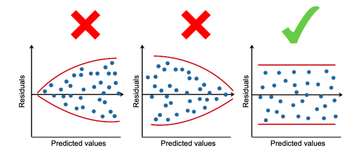
While summary statistics are a great way to compare models to one another at scale, figuring out whether our regression is working as expected from these metrics alone is still difficult. Therefore, a good approach in regression modeling is to also look at the distribution of the regression errors, called the residuals of our model. The distribution of the residuals gives us good visual feedback on how the regression model is performing.

A residual diagram plots the predicted values against the residuals as a simple scatterplot. Ideally, a residual plot should look like the following chart to back up the following assumptions:

• The points in the residual plot should be randomly scattered without exposing too much curvature (Linearity).

• The spread of the points across predicted values should be more or less the same for all predicted values (Homoscedasticity).

Residual plots will show you on which parts of your data the regression model works well and on which parts it doesn’t. Depending on your use case, you can decide whether this is problematic or still acceptable, given all other factors. Looking at the summary statistics alone would not give you these insights. Keeping an eye on the residuals is always a good idea when evaluating regression models.

After understanding how to evaluate regression models, let's move to classification models.

Evaluating Classification Models

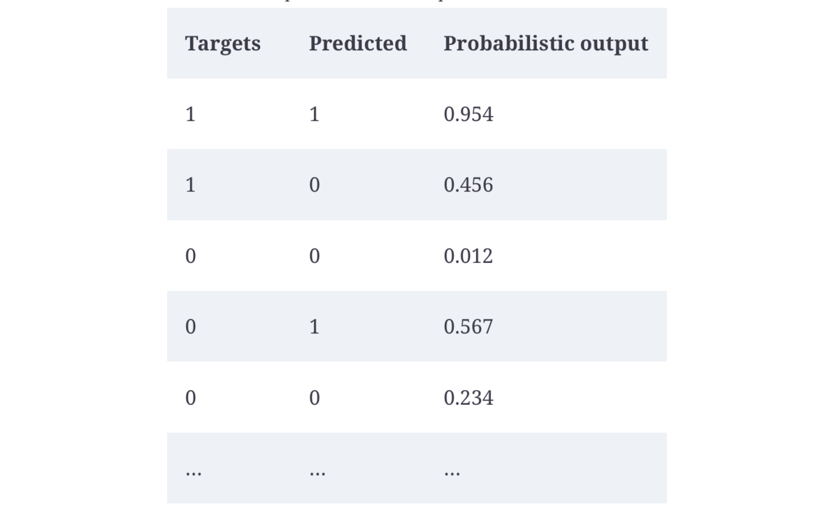
If the predicted values are not numeric but categorical, we can’t apply the regression metrics. Take a look at this table:

The table shows the true labels of a classification problem ("Targets") with the corresponding outputs ("Predicted" and “Probabilistic output” ) of a classification model.

If you look at the first four rows, you’ll see four things that could happen here:

• The true label is 1, and our prediction is 1 (correct prediction).

• The true label is 0, and our prediction is 0 (correct prediction).

• The true label is 1, and our prediction is not 1 (incorrect prediction).

• The true label is 0, and our prediction is not 0 (incorrect prediction).

The most popular way to measure the performance of a classification model is to display these four outcomes in a confusion table, or confusion matrix:

In our example, the confusion table tells us that there were 2,388 observations in total where the actual label was 0 and our model identified them correctly. We call these true negatives.

Likewise, for 2,954 observations both the actual and the predicted outcome had the positive class label (1) - true positives.

But our model also made two kinds of errors.

First, it wrongly predicted 558 negative classes to be positive. This is known as a type I error.

Second, the model incorrectly predicted 415 cases to be negative that were, in fact, positive. That's what we call type II errors.

(Statisticians were rather less creative in naming these things.)

With this information, we can calculate various metrics that serve different purposes:

Accuracy

The most popular metric you'll hear and see is accuracy. Accuracy describes how often our model was correct, based on all predictions.

It's the total number of correct predictions divided by the number of all predictions:

In our example. the accuracy is (2,388 + 2,954) / (2,954 + 2,388 + 558 + 415) = 0.8459.

Interpretation: Our model was correct in 84.59% of all cases.

Usage: Accuracy works only for balanced classification problems. Imagine we want to predict credit card fraud, which happens in only 0.1% of all transactions. If our model consistently predicts no fraud, it would yield an astonishing accuracy score of 99.9%. While this model has an excellent accuracy metric, it’s clear that this model isn’t useful at all.

That’s why the confusion matrix allows us to calculate even more metrics that are more balanced toward correctly identifying positive or negative class labels.

Precision

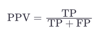
Precision, or positive predictive value (PPV), measures the proportion of true positives and is defined as follows:

In our example, the precision is 2,954 / (2,954 + 558) = 0.8411.

Interpretation: When the model labeled a data point as positive (1), it was correct 84% of the time.

Usage: Choose this metric if the costs of a false positive are very high and the costs of a false negative are rather low (e.g. when you want to decide whether to show an expensive ad to an online user).

Recall

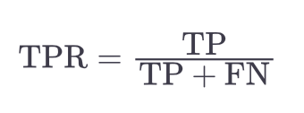
Recall (= sensitivity, true positive rate (TPR) is another metric that looks at the positive classes but with a different focus. It gives the percentage of all positive classes that were correctly classified as positive:

In our example, the recall would be 2,954 / (2,954 + 415) = 0.8768.

Interpretation: The model could identify 87.68% of all positive classes in the dataset.

Usage: Choose recall when the costs of missing these positive classes (false negatives) are very high (e.g., for fraud detection).

F-Score

If you still have an imbalanced classification dataset but don’t want to lean towards precision or recall, you could consider another commonly used metric called the F-score.

Despite its technical name, this metric is relatively intuitive as it combines precision and recall. The most popular F-score is the F1-score, which is simply the harmonic mean of precision and recall:

In our case, the F1-score would thus be 2 × (0.8411 × 0.8768) / (0.8411 + 0.8768) = 0.8586.

Interpretation: A higher F1-score indicates a better-performing model, but it isn’t as easily explained in one sentence as the previous metrics. Since the F1-score is the harmonic of precision and recall instead of the arithmetic mean, it will tend to be lower if one of these would be very bad. Imagine an extreme example with a precision of 0 and a recall of 1. The arithmetic mean would return a score of 0.5, which roughly translates to “If one is great, but the other one is poor, then the average is OK.” The harmonic mean, however, would be 0 in this case. Instead of averaging out high and low numbers, the F1-score will raise a flag if either recall or precision is extremely low. And that is much closer to what you would expect from a combined performance metric.

Usage: Choose the F1-score when you want to balance between precision and recall, or when you have an imbalanced classification dataset.

Evaluating Multiclassification Models

The metrics we used for binary classification problems also apply to multiclassification problems (which have more than two classes to predict).

For example, consider the following targets and predicted values:

• target_class = [1, 3, 2, 0, 2, 2]

• predicted_class = [1, 2, 2, 0, 2, 0]

The only difference between a binary and a multiclassification problem is that you would calculate the evaluation metrics for each class (0, 1, 2, 3) and compare it against all other classes.

The way you do that can follow different approaches, usually referred to as the micro and macro value.

Micro scores typically calculate metrics globally by counting all the total true positives, false negatives, and false positives together and only then dividing them by each other.

Macro scores, on the other hand, calculate precision, recall, and so forth for each label first and then calculate the average of all of them. These approaches produce similar, but still different, results.

For example, our dummy series for the four classification labels has a micro F1-score of 0.667 and a macro F1-score of 0.583. If you like, try it out and calculate the numbers by hand to foster your understanding of these metrics.

Neither of the micro or macro metrics is better or worse. These are just different ways to calculate the same summary statistic based on different approaches. These nuances will become more critical after you work on more complex multiclass problems.

Conclusion

Evaluating predictive models is a critical aspect of any data-driven decision-making process. In this guide, we've delved into some key evaluation metrics for both regression and classification models.

It's important to remember that no single metric is a silver bullet.

The choice of metric should always be guided by your specific use case, the nature of your data, and the cost implications of different kinds of errors.

This, coupled with a solid understanding of these metrics, will empower you to determine when your model's performance is sufficient, saving you from unnecessary complexity and computational cost.

Remember that there's always more to learn! We have not touched on performance metrics that consider probabilistic outputs, like AUC, or discussed advanced topics like model bias and fairness, which are increasingly important in ethical AI development.

Continue to explore, and feel free to reach out with any questions or topics you'd like to see covered in the future.

Happy modeling and see you next Friday!

Tobias

Resources

• [Book] Ch. 3 Machine Learning Fundamentals in AI-Powered Business Intelligence, O’Reilly 2022

• [Google Blog] Classification: ROC Curve and AUC

• [Azure Documentation] Evaluating Machine Learning Experiments

• [Video] Residual Analysis in Regression

Want to learn more? Here are 3 ways I could help:

1. Read my book: Improve your AI/ML skills and apply them to real-world use cases with AI-Powered Business Intelligence (O'Reilly).

2. Book a meeting: Let's get to know each other in a coffee chat.

3. Follow me: I regularly share free content on LinkedIn and Twitter.